Inside Quantization Aware Training

Introduction

Real-world applications of Deep Neural Networks are increasing by the day as we are learning to make use of Artificial Intelligence to accomplish various simple and complex tasks. However, the problem with Deep Neural Networks is that they involve too many parameters due to which they require powerful computation devices and large memory storage. This makes it almost impossible to run on devices with lower computation power such as Android and other low-power edge devices. Optimization techniques such as Quantization can be utilized to solve this problem**.** With the help of different quantization techniques, we can reduce the precision of our parameters from float to lower precision such as int8, resulting in efficient computation and less amount of storage. One of the most optimal quantization techniques is Quantization-Aware Training. In this post, we will understand its mechanism in detail.

What is Quantization-Aware Training?

As we move to a lower precision from float, we generally notice a significant accuracy drop as this is a lossy process. This loss can be minimized with the help of quant-aware training. So basically, quant-aware training simulates low precision behavior in the forward pass, while the backward pass remains the same. This induces some quantization error which is accumulated in the total loss of the model and hence the optimizer tries to reduce it by adjusting the parameters accordingly. This makes our parameters more robust to quantization making our process almost lossless.

How is it Performed?

We first decide on a scheme for quantization. It means deciding what factors we want to include to convert the float values to lower precision integer values with minimum loss of information. In this article, we will be using the quantization scheme used in [1] as a reference. So we introduce two new parameters for this purpose: scale and zero-point. As the name suggests scale parameter is used to scale back the low-precision values back to the floating-point values. It is stored in full precision for better accuracy. On the other hand, zero-point is a low precision value that represents the quantized value that will represent the real value 0. The advantage of zero-point is that we can have a wider range for integer values even for skewed tensors. So real values (r) could be derived from quantized values (q) in the following way:

Here S and Z represent scale and zero-point respectively.

We introduce something known as FakeQuant nodes into our model after every operation involving computations to obtain the output in the range of our required precision. A FakeQuant node is basically a combination of Quantize and Dequantize operations stacked together.

Quantize Operation

Its main role is to bring the float values of a tensor to low precision integer values. It is done based on the above-discussed quantization scheme. Scale and zero-point are calculated in the following way:

The main role of scale is to map the lowest and highest value in the floating range to the highest and lowest value in the quantized range. In the case of 8-bit quantization, the quantized range would be [-128,127].

here fₘₐₓ and fₘᵢₙ represent the maximum and minimum value in floating-point precision, qₘₐₓ and qₘᵢₙ represent the maximum value and minimum value in the quantized range.

Similarly, we can find the zero-point by establishing a linear relationship between the extreme floating-point values and the quantized values.

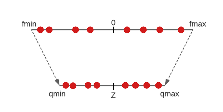
Considering we have coordinates of two points of a straight line (qₘᵢₙ,fₘᵢₙ) and (qₘₐₓ,fₘₐₓ), we can obtain its equation in the form of y = mx +c, x being the quantized values and y being the real values. So to get the mapping of 0 in the quantized domain, we just find the value of x with y=0. On solving this we would get:

But what if 0 doesn’t lie between fₘₐₓ and fₘᵢₙ, our Zero point would then go out of the quantization range. To overcome this, we can set Z to qₘₐₓ or qₘᵢₙ depending on which side it lies on.

Now we have everything for our Quantize operation and we can obtain quantized values from floating-point values using the equation:

Further, we will convert it back to the floating domain using the Dequantize operation to approximate the original value but it will induce some small quantization loss that we will use to optimize the model.

Dequantize Operation

To obtain back the real values we put the quantized value in Equation 1, so that becomes:

Creating a Training Graph

Now that we have defined our FakeQuant nodes, we need to determine the correct position to insert them in the graph. We need to apply Quantize operations on our weights and activations using the following rules:

• Weights need to be quantized before they are multiplied or convolved with the input.
• Our graph should display inference behavior while training so the BatchNorm layers must be folded and Dropouts must be removed. Details on BatchNorm folding can be found here.
• Outputs of each layer are generally quantized after the activation layer like Relu is applied to them which is beneficial because most optimized hardware generally have the activation function fused with the main operation.
• We also need to quantize the outputs of layers like Concat and Add where the outputs of several layers are merged.
• We do not need to quantize the bias during training as we would be using int32 bias during inference and that can be calculated later on with the parameters obtained using the quantization of weights and activations. We will discuss that later in this post.

Scales and Zero-points of weights are determined simply as discussed in the previous section. To determine scales and zero-points of activations we need to maintain an exponential moving average of the max and min values of the activation in the floating-point domain so that our parameters are smoothened over the data obtained from many images.

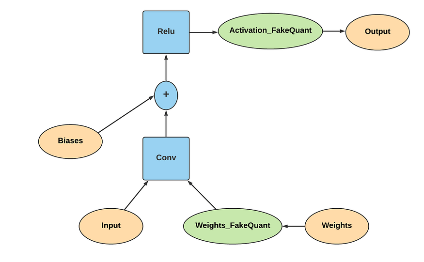
So the fake quantize operations are inserted in the graph as shown below.

Now that our graph is ready, we need to prepare it for training. While training we have to simulate the quantization behavior only in the forward pass to induce the quantization error, the backward pass remains the same and only the floating-point weights are updated during training. To achieve this in TensorFlow we can take the help of the @custom_gradient decorator. This decorator helps us define our own custom gradient for any operation.

Creating an Evaluation or Inference Graph

Now that we have completed our training and our parameters are now tuned for better low precision inference, we need to obtain a low precision inference graph from the obtained training graph to run it on optimized hardware devices.

• First, we need to extract the quantized weights from the above model and apply the Quantize operation to the weights obtained during quant-aware training.
• As our optimized function will be accepting only low precision inputs, we also need to quantize our input.

Now let’s derive how we can obtain our quantized result using these quantized parameters.

Suppose we assume convolution as a dot operation.

Using Equation 1, It can also be written as:

To obtain the quantized value q₃, we rearrange the equation to be:

In this equation, we can compute (S₁S₂)/S₃ offline before the inference even begins and this can be replaced with a single multiplier M.

Now to further reduce it to Integer-only arithmetic, we try to break down M into two integer values. M always lies between 0 and 1, so it can be broken down into this form.

Using this equation we can obtain the integer values of M₀ and n which will act as a multiplier and a bit-wise shifter values respectively. Obviously, this step is not required if we can perform float multiplication on our hardware.

Also, we need to modify our bias accordingly as our multiplier would also be affecting it. Hence, we can obtain our int32 quantized bias for inference using the following equation:

Now that we have all our ingredients, we can create our low precision inference graph which would look something like this.

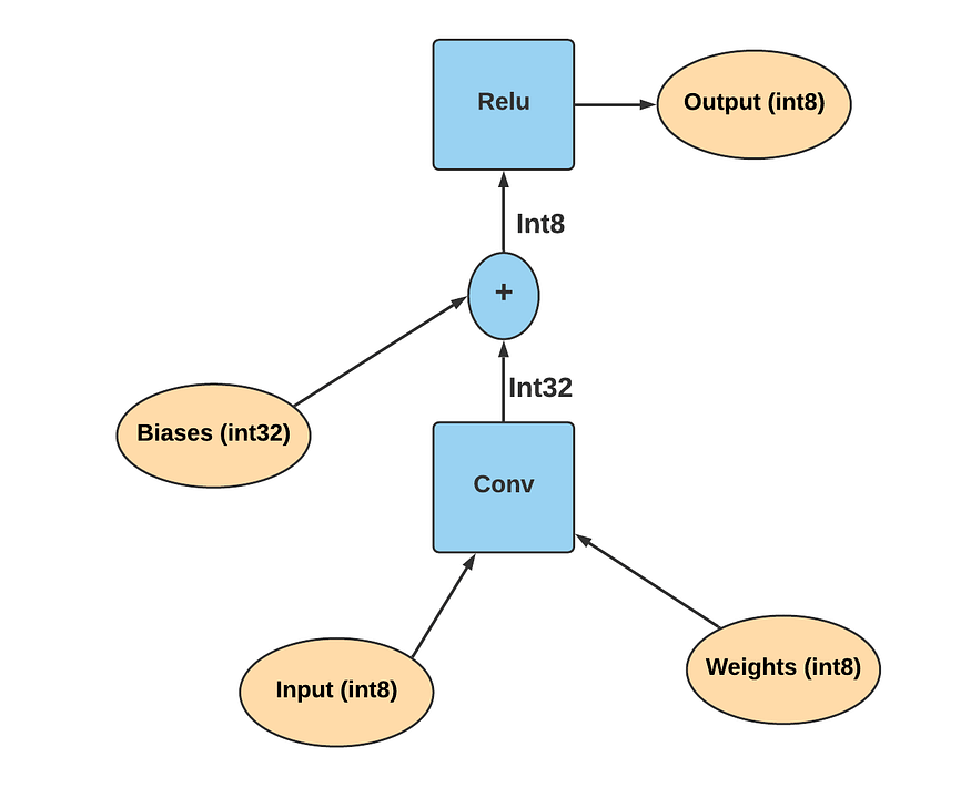
It is up to us if we want to take the quantized range as signed or unsigned. In the above graph, it is considered unsigned.

Is Quantization Aware Training worth the effort?

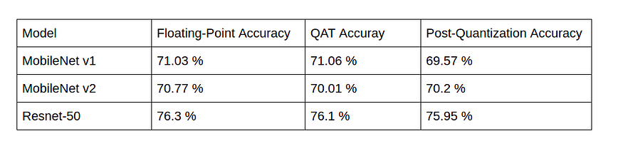
As we already know the importance of quantization and also knowing that Post-Quantization could be very lossy sometimes, Quantization-Aware training is our best bet. The following table shows the results of Quant-Aware training with some of the popular and complex neural network architectures. We can observe that the accuracy drop is negligible in this mode of quantization.

Also, we do not need to worry about implementing such a complex mechanism on our own as Tensorflow provides a well-defined API for this purpose. You can learn about it from here.

References

[1] Benoit Jacob, Skirmantas Kligys, Bo Chen, Menglong Zhu, Matthew Tang, Andrew Howard, Hartwig Adam and Dmitry Kalenichenko, Quantization and Training of Neural Networks for Efficient Integer-Arithmetic-Only Inference[2017]

[2] https://blog.tensorflow.org/2020/04/quantization-aware-training-with-tensorflow-model-optimization-toolkit.html

[3]https://intellabs.github.io/distiller/algo_quantization.html

[4] https://scortex.io/batch-norm-folding-an-easy-way-to-improve-your-network-speed/